
 The lecture encyclopedia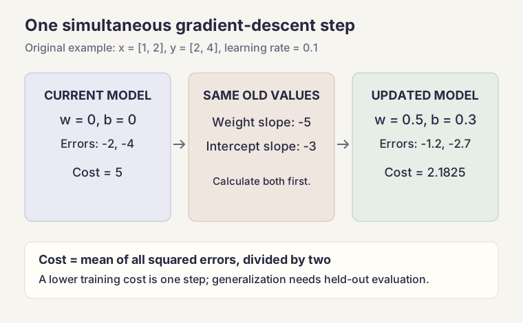
A regression model predicts a number. Evaluating that prediction and finding the model's parameters are related tasks with different purposes. Evaluation measures error on selected examples. Gradient descent repeatedly changes parameters to reduce a chosen training cost. This session revisits evaluation before introducing optimization and multiple input features.
Read thresholds and generalization for the preceding discussion of independent evaluation. A smaller training cost does not, by itself, establish better predictions on new examples.
Measure numeric error without cancellation #
Let an error be the predicted value minus the actual value. Predictions of 11 and 17 for actual values of 10 and 20 give errors of 1 and -3. Their average is -1, which hides the size of the mistakes: one prediction is too high and the other is too low.
Mean squared error, or MSE, averages the squared errors. Here it is (1² + (-3)²) / 2 = 5. Mean absolute error, or MAE, averages their magnitudes: (1 + 3) / 2 = 2. Root mean squared error, or RMSE, is √5, approximately 2.24. MAE and RMSE use the target's original units; MSE uses squared units. Squaring also gives a relatively large mistake more influence.[1]
Precision, recall, accuracy, and ROC AUC describe classification tasks. For a numeric target, choose an appropriate regression metric. Cross-validation supplies held-out predictions; a metric still measures the quality of those predictions. A model that learns training noise can overfit, while a model too restrictive to represent the relationship can underfit.
Connect a prediction to its cost #
With one input feature, the prediction is ŷ = wx + b. The input x is an observed measurement; w is the learned weight, and b is the learned intercept. For the possum example discussed in the session, body length is the input and head length is the target. The following calculations use an original two-point example rather than that dataset.
The notebook's corrected cost is one half of the mean squared error across all examples:
J(w, b) = [sum of (wxᵢ + b - yᵢ)²] / (2m), where m is the number of examples.
Compute a prediction for every matching input and target, square every error, then average and divide by two. The earlier single-example description does not produce the aggregate cost required by this notebook. The factor of one half simplifies the derivative; multiplying a cost by a positive constant does not change which parameters minimize it, although it changes gradient magnitudes and the suitable step size.
For nonempty, same-length one-dimensional NumPy arrays, the calculation can be written as follows. NumPy's mean performs the averaging.[2]
import numpy as np

def regression_cost(x, y, w, b):
    prediction = w * x + b
    errors = prediction - y
    return np.mean(errors ** 2) / 2
The function evaluates the parameters it receives. Resetting w or b inside it would erase the caller's candidate model. Array shapes also matter: use aligned vectors so subtraction does not accidentally broadcast into a matrix of unrelated comparisons.
Take one downhill step #
Think of the cost as a surface over parameter choices. A gradient records the cost's local slopes. Subtracting a small multiple of those slopes changes the parameters in a downhill direction. The learning rate α controls the step size. Compute all proposed parameters from the same current values, then assign them together.[3]
For the half-MSE cost, the slope for w is the average of error times x; the slope for b is the average error. In the original example, use two observations: x values 1 and 2, with targets 2 and 4. Start with w = 0 and b = 0.
| Quantity | Calculation | Result |
|---|---|---|
| Predictions | 0 × 1 + 0; 0 × 2 + 0 | 0; 0 |
| Errors | 0 - 2; 0 - 4 | -2; -4 |
| Current cost | (4 + 16) / 4 | 5 |
| Slope for w | ((-2) × 1 + (-4) × 2) / 2 | -5 |
| Slope for b | (-2 + -4) / 2 | -3 |
With α = 0.1, the proposed weight is 0 - 0.1 × (-5) = 0.5, and the proposed intercept is 0 - 0.1 × (-3) = 0.3. Both slopes came from the original zero parameters. The new predictions are 0.8 and 1.3, giving cost (1.44 + 7.29) / 4 = 2.1825. One step reduced cost from 5 to 2.1825; it did not finish fitting the line.
Updating w first and using that new value while calculating b changes the procedure. Store both proposed updates temporarily when implementing the simultaneous algorithm.
Interpret learning rates and convergence #
A tiny learning rate may make useful progress slowly. A large rate may overshoot, oscillate, or diverge. Monitor the actual cost history rather than assuming every chosen rate will work. A fixed iteration count limits runtime; it is not proof that the parameters have converged.
Unregularized linear regression with squared-error cost has a convex objective. Its surface has no separate, inferior local valleys. Correlated or redundant features can still make the best parameters nonunique. Other model families can have nonconvex surfaces, so a picture of several local minima should not be confused with this squared-error linear model.
Features on very different scales can make optimization difficult. Fit any scaling transformation using training data, then apply that same transformation to held-out data. Recomputing it from test data compromises independence. Batch gradient descent uses the whole training set for a step; stochastic gradient descent uses individual examples, and mini-batch variants use subsets.[4]
Give each feature a weight #
Multiple linear regression predicts one numeric target from several input features. For one example, x is now a vector. Each feature has a corresponding weight; b remains a single intercept. The prediction is their dot product plus b.[5]
For a simple original example, let x = [2, 3], w = [4, -1], and b = 5. The prediction is 2 × 4 + 3 × (-1) + 5 = 10. There are two features and two weights, but only one prediction. A capital X commonly denotes the table containing many examples.
x = np.array([2.0, 3.0])
w = np.array([4.0, -1.0])
b = 5.0
prediction = np.dot(x, w) + b
For these one-dimensional arrays, multiplication with * produces separate elementwise products; np.dot adds the pairwise products into the required weighted sum. More features add parameters and may add useful information or noise. Compare held-out performance before concluding that a larger feature set is better.
Least squares also admits direct numerical solution methods. A library's ordinary LinearRegression estimator need not use gradient descent; scikit-learn documents its least-squares solver separately. Understand the objective and the optimizer as separate choices.[6]
Practice with explained answers #
Why is the notebook's cost half the MSE? The definition includes a factor of one half. It keeps the same minimizer as MSE while simplifying derivatives. Report ordinary MSE without this factor when MSE is the requested evaluation metric.
Can a training cost decrease while held-out predictions get worse? Yes. Optimization can improve training fit while a flexible model learns noise. Use independent evaluation to check generalization.
In one simultaneous step, should the b slope use the newly assigned w? No. Calculate both slopes from the parameters at the start of that step.
Does using four features mean predicting four outcomes? No. This model combines four weighted inputs to predict one target. Predicting several outputs is a different extension.