Thresholds, generalization, and responsible model evaluation

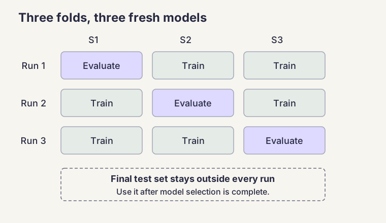
A classifier can rank examples well and still make the wrong decisions for its intended use. Evaluation asks both whether a model learns a pattern that survives new data and whether its mistakes are acceptable. This lecture builds on confusion matrices, precision, and recall to connect decision thresholds, independent testing, model complexity, and the people affected by predictions.

Follow the ideas in this order: decide what counts as a positive case, inspect the mistakes at a chosen threshold, test on unseen examples, and then choose how much flexibility the model needs. A high score becomes useful evidence only when you know what was measured and how the evaluation stayed independent.

From a score to a decision #

A binary classifier distinguishes two categories. For a handwritten-digit task, let positive mean “this image is a five” and negative mean “this image is not a five.” Many models first produce a numerical score. A threshold turns that score into a label: a score at or above the threshold receives the positive label.

A score is not automatically a well-calibrated probability. The threshold rule can still be applied to a ranking score, but “0.8” does not necessarily mean an 80 percent chance that the prediction is correct. Separate what the model calculates from what you are entitled to infer.

A true positive (TP) is a real five called a five. A false positive (FP) is another digit called a five. A false negative (FN) is a real five that the model misses. A true negative (TN) is another digit correctly rejected. These four counts form the confusion matrix.

Precision is TP / (TP + FP): among the images called five, how many are actually five? Recall is TP / (TP + FN): among the actual fives, how many did we find? The denominators describe different groups. F1 combines the two using 2PR / (P + R), where P is precision and R is recall. A zero denominator needs an explicit reporting convention rather than ordinary division.^[1]

Work through a threshold change #

Suppose the dataset contains six actual fives. At the first threshold, the model calls five images positive, of which four are fives.

1. Four correctly identified fives give TP = 4.
2. One incorrect positive gives FP = 1.
3. Two missed fives give FN = 2.
4. Precision is 4 / 5 = 0.80; recall is 4 / 6 ≈ 0.667.

Now lower the threshold. Eight images qualify as positive, including all six fives. TP becomes six, FP becomes two, and FN becomes zero. Precision is 6 / 8 = 0.75; recall is 6 / 6 = 1.00.

The model found two additional fives and admitted one additional false alarm. That is the concrete trade-off hidden inside the percentages. F1 rises from 8 / 11 ≈ 0.727 to 12 / 14 ≈ 0.857, but even that improvement does not tell us whether the extra false alarm is acceptable.

Raising the threshold makes the rule more selective. It cannot add positive predictions when the scores and comparison rule stay fixed. Recall therefore cannot rise as the threshold rises on this fixed dataset; precision can fluctuate because the newly excluded examples may include either correct or incorrect predictions. Better data or a better model can improve both measures, so this threshold trade-off is not a universal limit on improvement.

Read ROC and precision-recall curves #

A precision-recall curve compares the pairs produced by different thresholds. It helps show how much precision is lost while finding more positives. Inspect the region that matches the application's requirements rather than choosing a visually attractive point.

The receiver operating characteristic, or ROC, uses a different horizontal axis. The vertical axis is true positive rate, which equals recall. The horizontal axis is false positive rate, FP / (FP + TN): the fraction of actual negatives that became false alarms. A useful operating point has high true positive rate and low false positive rate, toward the upper-left corner.^[1]

Specificity, or true negative rate, is the fraction of actual negatives correctly rejected. It equals one minus the false positive rate. Sensitivity is another name for recall or true positive rate.

False positive rate is not one minus precision. The former divides by actual negatives; the latter describes predicted positives. In the digit example, we know FP but have not specified TN, so we cannot compute a numerical false positive rate from the supplied counts alone.

Area under the ROC curve, usually called ROC AUC, summarizes ranking performance across thresholds. Perfect separation gives an AUC of one; random ranking has expected AUC around one half. AUC does not choose a threshold, establish probability calibration, or show that every group receives equally reliable predictions. On an imbalanced task, inspect precision and recall alongside ROC rather than assuming a single summary settles usefulness.

Keep evaluation independent #

Overfitting happens when a model fits accidental features of its training sample so closely that it performs poorly on new examples. Underfitting happens when it fails to capture useful structure, often because it is too restrictive. Excellent training performance alone cannot distinguish learning a general pattern from memorizing quirks.

Separate three roles. Training data fit the model's parameters. Development validation guides choices such as tree depth, model family, and decision threshold. A final test set estimates performance after those choices are finished. Names vary between demonstrations; the essential question is whether an evaluation result influenced a subsequent choice.

If you inspect a test score, change the model, and repeat until that score looks good, the set has become part of development. Preserve another untouched evaluation set when possible. Preprocessing can leak information too: fit data-dependent transformations using training data within each split, then apply them to held-out data.^[2]

For ordinary independent classification examples, an illustrative split is:

from sklearn.model_selection import train_test_split

X_dev, X_final, y_dev, y_final = train_test_split(
    X, y, test_size=0.33, random_state=42, stratify=y
)

X contains the features and y the matching target labels. The four returned collections keep each selected example aligned with its answer. test_size=0.33 reserves about one third for final evaluation; random_state=42 makes this illustrative split reproducible; stratify=y aims to preserve class proportions when enough examples exist. Here X_dev is still development data, not automatically a completed training set.

Random splitting is appropriate only when it matches the task. Time-ordered forecasts and repeated measurements of the same subject need splits that respect time or groups. Taking the first rows of a species-sorted file can also create an unrepresentative split. Neither a convenient function nor a fixed seed proves independence.

Rotate folds without carrying learning across runs #

Cross-validation divides development data into k folds. In each run, a fresh model is fitted on k minus one folds and evaluated on the remaining fold. For three folds:

1. Train on S2 and S3; evaluate on S1.
2. Train on S1 and S3; evaluate on S2.
3. Train on S1 and S2; evaluate on S3.

Each example is held out once and used for training in two separate runs. The runs do not successively improve one fitted model. Carrying its learning from the first run into the second would expose evaluation examples to earlier training.

For equally weighted fold scores of 0.80, 0.75, and 0.85, the mean is (0.80 + 0.75 + 0.85) / 3 = 0.80. Inspect variation too: a mean can conceal a fold with much worse results. Five or ten folds are common choices; leave-one-out uses one held-out example per run and can be expensive. Keep the final evaluation set outside these model-selection runs.^[2]

Choose flexibility using held-out performance #

A hyperparameter controls how a model is built, rather than being a fitted coefficient. A tree's maximum depth is one example. Compare candidate settings using development evaluation. A flexible model often fits training data better, but held-out performance may first improve and then deteriorate as flexibility begins capturing noise.

The bias-variance trade-off describes two sources of difficulty. A restrictive model may systematically miss the useful relationship: high bias. A highly flexible model may change sharply when the training sample changes: high variance. These tendencies help diagnose behavior; they are not rigid labels that classify every error.

A degree-zero polynomial predicts a constant. A degree-one polynomial draws a straight line. Higher degrees allow more bends. With ten distinct input points, a degree-nine polynomial can interpolate all ten observations, including their noise. Passing through those observations does not establish reliable predictions between or beyond them. More useful data can reduce sensitivity to a small sample, but more data cannot make a constant model represent a curved relationship.

Training, development, final-test, and deployment scores do not have a guaranteed descending order. Sampling variation can change the order, and new conditions can change the task. Diagnose the actual results rather than assuming a fixed hierarchy of percentages.

Prune a decision tree #

A decision tree can become overly specific by repeatedly splitting small groups. Pre-pruning limits growth, for example through maximum depth or a minimum number of examples required for a leaf. This avoids building some unnecessary branches, but an early stop can also prevent useful deeper structure from being discovered.

Post-pruning starts with a larger tree and simplifies it. In the classroom's conceptual description, a selected subtree is replaced by a leaf predicting the majority class among examples that reach it. Evaluate the simplified candidate on development data, and keep a change when the chosen criterion supports it. Specific implementations may optimize a complexity penalty; scikit-learn offers minimal cost-complexity pruning through ccp_alpha.^[3]

Suppose a branch divides only a handful of examples into nearly pure leaves. Ask whether those divisions improve performance on examples outside the training sample. Purity on a tiny training group is weak evidence by itself. Pruning trades some training fit for a simpler model that may generalize better; it does not guarantee improvement on every test set.

Connect mistakes to human consequences #

Choose an application-specific standard before declaring automation useful. A false alarm in a digit exercise is an incorrect label; a false suspicion in a welfare process may trigger an intrusive investigation. The numerical categories are similar, but their consequences differ.

Lighthouse Reports' investigation of Rotterdam's welfare risk system describes how scoring and personal characteristics could shape investigation decisions. It gives a concrete reason to examine error burdens and communicate limitations, rather than treating a functioning classifier as sufficient justification for use.^[4] A score identifying a case for review is not proof of fraud.

Compare the proposed process with a relevant baseline, inspect performance for affected groups, and explain which decisions the evidence supports. Monitor performance after deployment because the population and process can change. The responsibility is to connect the mathematical evaluation to the actual action taken on its basis.

Practice with explained answers #

Why can we calculate recall but not false positive rate for the six-fives example? We know TP and FN, giving the number of actual positives. We do not know the number of actual negatives, which is FP plus TN.

A model earns 100 percent training accuracy and 68 percent held-out accuracy. What should you investigate? Overfitting is a plausible explanation, but also check leakage, the split, sample sizes, and differing data conditions. Try a less flexible model or better training data, then compare using development evaluation. The gap is evidence to investigate, not proof of one cause.

You choose tree depth using three-fold validation, then evaluate once on an untouched final set. Which score guided the choice? The cross-validation score did. The final score estimates the chosen procedure's performance; using it to choose another depth would turn it into development evidence.

Does a larger AUC remove the need for a threshold decision? No. Ranking and taking action are separate steps. Decide the tolerable mix of false alarms and missed cases, inspect that operating point, and explain its consequences.