
 The lecture encyclopedia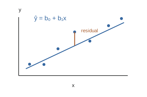
Simple linear regression predicts a numeric response from one numeric input using a straight line. It extends the preparation workflow from understanding attributes and distances to fitting a model whose predictions can be evaluated quantitatively.
Inputs and responses #
The explanatory variable is commonly written x; the observed response is y. The model's prediction is ŷ = wx + b, where w is the slope and b is the intercept. In a measurement example, one body measurement might predict another. Choosing which variable is the input changes the question being answered.
Slope and intercept #
The slope describes the predicted change in the response for a one-unit increase in the input. The intercept is the prediction at input zero. It may have little practical interpretation when zero lies far outside the observed range.
For the illustrative model ŷ = 2x + 3, an input of 4 yields a prediction of 11. If the observed response is 13, the residual y - ŷ is 2. A prediction and an observation are different quantities even when a fitted model makes them close.
Mean squared error #
Mean squared error averages squared residuals: MSE = Σ(yᵢ - ŷᵢ)² / n. Squaring prevents positive and negative errors from canceling and gives larger errors greater influence. For residuals 1, -1, and 2, MSE is (1 + 1 + 4) / 3 = 2.[1]
Fitting chooses model parameters to improve an objective such as this error. A low training error alone is not enough; evaluate the fitted relationship on observations that did not determine its parameters.
Preparation still matters #
Attribute types determine whether numeric operations are meaningful. Missing values and outliers affect a fit, and differences in measurement units affect coefficient interpretation. Python variables bind to typed objects, so converting text measurements and checking the resulting schema are part of modeling rather than separate clerical tasks.
Limits of a line #
A linear model describes a particular form of association. It does not establish causation, and extrapolating beyond the observed input range can be unreliable. A scatterplot and residual inspection help reveal curvature, unusual observations, or changing error patterns that a single score conceals.