Searching, sorting, and multidimensional arrays

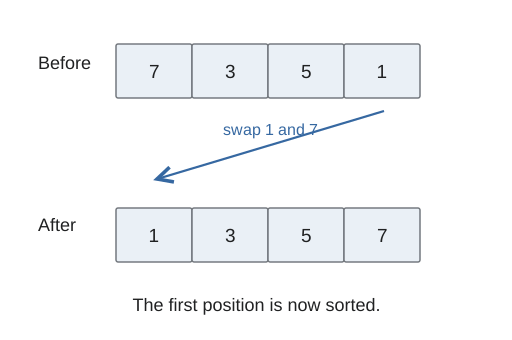
Searching, inserting, removing, and sorting all operate on stored elements, but they change different things. A search finds a position. Insertion and removal change the active count. Sorting changes order while preserving the values and count. A clear invariant tells you what must remain true after each operation.

Review CS1: searching and sorting and CS1: grids for the starting ideas. This lecture connects the steps of those operations to array bounds and intermediate states.

Search returns a position, not a truth value #

A linear search starts at the first active element and compares one value at a time with a target. Suppose the active sequence is four, one, three and the target is one. The comparison at index zero fails. The comparison at index one succeeds, so the search returns one as the position.

If no comparison succeeds, the function needs an explicit not-found result. A negative sentinel is one possible interface. The caller must check it before indexing the array. Index zero is a successful position, even though converting the integer zero directly to bool produces false. A negative not-found sentinel is nonzero, so blindly treating the result as a Boolean reverses the intended meaning in important cases.

The active count limits the search. Unused capacity is not another set of observations to inspect. An empty active range produces not-found without reading any element.

Insert and remove without losing values #

To insert in the middle of a partially filled array, first make sure capacity exceeds the active count. The insertion position must also be between zero and the active count, inclusive; spare capacity alone does not validate an arbitrary position. Then move existing elements one position to the right, starting at the end. Moving right to left preserves each old value before its original slot is overwritten.

For four, one, three, inserting nine at index one starts by moving three to index three, then one to index two. Four stays at index zero. The slot at index one can now receive nine, giving four, nine, one, three. The active count grows from three to four. Moving left to right would overwrite a value before you had copied it out.

For removal, require an existing active index: at least zero and strictly below the active count. Removal does the reverse movement. To remove index one from that four-element sequence, move the later one left to index one and three left to index two, then reduce the active count to three. The old final slot remains allocated but is no longer active. Removal changes logical size, not physical capacity.

Selection sort settles one prefix position #

Selection sort divides the sequence into a finished prefix and a remaining suffix. On each pass, find the smallest value in the remaining part and swap it into the next prefix position.

For [4, 1, 3], the first pass finds one at index one. Swapping it with index zero gives one, four, three. The first position is now settled. The second pass examines four and three, finds three smaller, and swaps those positions. The result is [1, 3, 4].

The important intermediate value is the minimum's index. Update that index while scanning, then perform the needed exchange after the scan. You are not repeatedly swapping every smaller value you encounter. The count never changes, and every original value remains present.

Bubble sort settles a suffix #

Bubble sort compares adjacent pairs. If a pair is out of order, exchange it. For four, one, three, compare four with one and swap, giving one, four, three. Then compare four with three and swap, giving one, three, four. The largest value has moved to the final position.

Later passes can omit the settled suffix. If an entire pass makes no exchanges, every compared adjacent pair was already ordered, so an optimized implementation can stop. A single pair requiring no swap does not establish that the whole sequence is sorted.

Ordinary selection sort and bubble sort generally require a number of comparisons growing quadratically with the element count. They are useful for understanding the movement of elements, while larger applications usually use a suitable library algorithm.

Give each dimension its own bound #

A two-dimensional array identifies a cell by row and column. For int grid[2][3], row indexes are zero and one; column indexes are zero, one, and two. A third dimension adds another coordinate and usually another nested loop.^[1]

for (int row = 0; row < 2; ++row) {
    for (int column = 0; column < 3; ++column) {
        grid[row][column] = row + column;
    }
}

Follow the outer loop first. At row zero, the inner loop assigns the cells zero, one, and two. The inner loop then finishes. At row one, a fresh inner traversal assigns one, two, and three. The row bound is two and the column bound is three; using one number for both would skip cells or step outside one dimension.

When this built-in multidimensional array is passed to a function, the remaining dimension information is needed to interpret the layout. A row contains three integers, so advancing to the next row must account for three elements. A pointer-based collection of separately allocated rows is a different representation, discussed later.

Practice and explanation #

Why does insertion shift toward the right from the final active element first? The destination slot is free before each source value is copied, so none of the still-needed sources is lost. Why does sorting leave used unchanged? It rearranges the same active observations; it neither appends nor removes one.

For the grid above, is row one, column three valid? No. Row one exists, but column three is outside the three-column range. Validate each coordinate separately.